
Near-real time monitoring system: Brief overview to Gaussian process state space models GPSS
Published:
Start (block 1)
The monitoring algorithm starts from the latest system state obtained in block 10. This is, the system state estimated at time k is fed back to begin a new estimation becoming then the state at k-1.
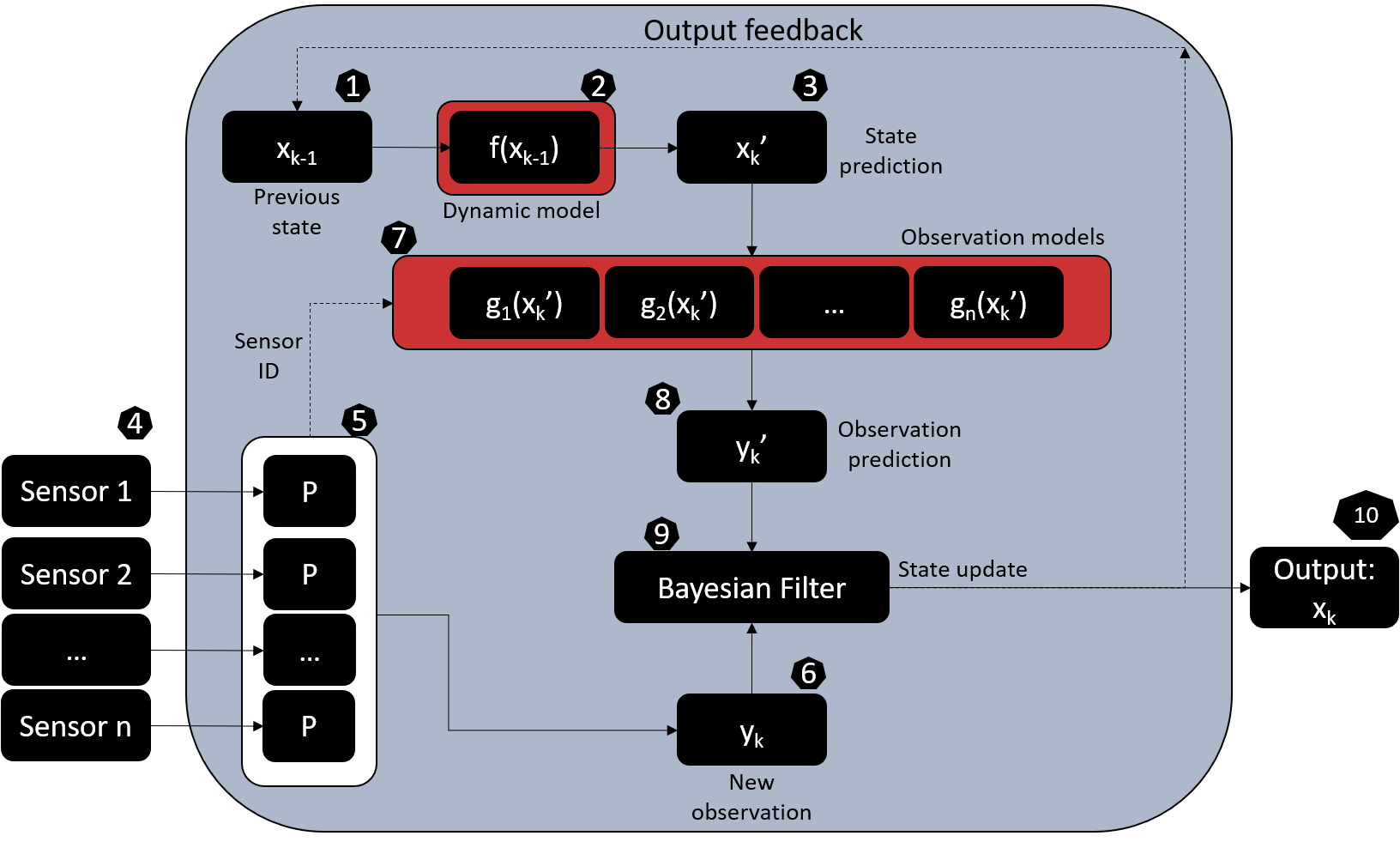
Dynamic model and state prediction (Blocks 2 and 3)
The dynamics of evolution of the state variables are represented by the probabilistic transition model specified by:
In equation (1) the system state at a given date k can be estimated as a function of the previous state xk-1 using the non-linear function f(.) and considering the additive gaussian system noise qk – N (0, Qk) accounting for the model uncertainty when making predictions. Note that the non-linear function f(.) represents the evolution rule of the dynamical system, which is a function that describes what future states follow from the current state. This can be seen as a stochastic differential equation and be learned by approximating it with a Gaussian process regression as proposed here. A future post will present the python code to implement this operation. Note that the transition model of equation (1) results in the conditional probability distribution P (xk | xk-1). In the blocks 3 and 4 the state is represented with the vector xk’ since it is not yet the estimated current state but our prediction of it based on the previous state.
Observation pre-processing and feature extraction (blocks 4 to 6)
New vector of observations ready (Block 6)
After pre-processing the raw sensor measurements the system observables are ready to be introduced in the tracking algorithm (Block 9).
Observations prediction (Blocks 7 and 8)
The E-dimensional random vector of sensor observations yk can be predicted as a function of the system state xk by means of the observation model:
State update
In order to achieve near-real time monitoring a Bayesian Filtering Framework (BFF) is used under which after every new observation at time k, we update our belief of the hidden system state xk considering from the first to the latest available observations acquired so far (y1:k) (assuming Markov property), regardless of the sensor that provides the acquisition. This belief is represented by the posterior probability distribution P(xk | y1:k) which in a BFF is estimated by recursively solving the prediction and update Bayesian filtering equations. Depending on the assumptions regarding the state distribution and the way of solving the Bayesian equations, the filter can become a non-linear Kalman filter or a Particle filter (a sequential Monte Carlo based sampling technique).
