In this post we will explore a flood mapping application from freely available remote sensing imagery. Specifically we will use Synthetic Aperture Radar data from the Sentinel-1 satellite.

Part of the ideas described in this post are based on this tutorial and this post. In this case, however, we will do it directly from QGIS using the python EE plug-in (link) which allows us to combine all the advantages of the google Earth Engine (GEE) platform to retrieve the already pre-processed satellite images with a very powerful and open source geospatial analysis software. We can then easily add to our project other shapefiles, raster and ground truth (csv files) data as well as exploit all the data analysis tools provided by python packages, i.e. numpy, pandas, matplotlib, sklearn, etc.

We will also see how with minimal modifications to our code we can readily analyse very different test sites and will see as examples the floods registered in Myanmar in 2015 using the same example as in here but without the pre-processing and in the river Severn, near Shrewsbury in England, at the beginning of this year (2020).

You can find the code for this post here

Here is a quick look of the results obtained following the steps mentioned below

Getting ready

Before we begin, we need to ensure that we have installed both the QGIS plug-in as explained here and the Google Earth Engine python API. We also need to provide our credentials to GEE so that we can access the satellite data with our account details. For more info about this have a look at this previous post. Now we need to open the python console in QGIS by clicking in “plugins, python console”. After that, the console appears, and we need to click on the “show editor” button where we will be adding the required python code.

(image of empty console)

Imports

import ee
from ee_plugin import Map
import time
from datetime import datetime

Preliminary functions

First of all we will define a couple of useful functions that will be used later in our code. We start with a function to obtain the Sentinel-1 images from GEE based on parameters such as the dates and area of interest, the desired radar backscatter polarisation (VH, VV or VH and VV), and the acquisition geometry (ascending or descending pass and orbit number). The python code with the corresponding code looks like this:

def get_Sentinel1_img(Latitude,Longitude,date1, date2,Direction,orbit_No):
    sentinel1 = (ee.ImageCollection('COPERNICUS/S1_GRD')
            .filterDate(date1, date2)
            .filter(ee.Filter.listContains('transmitterReceiverPolarisation', 'VV'))
            #.filter(ee.Filter.listContains('transmitterReceiverPolarisation', 'VH'))
            .filter(ee.Filter.eq('instrumentMode', 'IW'))
            .filter(ee.Filter.eq('orbitProperties_pass', Direction))
            .filter(ee.Filter.eq('relativeOrbitNumber_start', orbit_No))); 
              
    sentinel1 = sentinel1.filterBounds(ee.Geometry.Point(float(Longitude),float(Latitude)))
    
    recent = sentinel1.sort('system:time_start', False)
    lista = recent.toList(20)
    sentinel1_info=lista.getInfo()
    Images_in_collection=[]
    for i in range(len(sentinel1_info)):
        Images_in_collection.append(sentinel1_info[i]['id'])
    img_ID=Images_in_collection[0]
    img_ = ee.Image(Images_in_collection[0])
    return(img_,img_ID)

Now we will define a function that allows us to extract the date of the retrieved image from the title. The name conventions for a Sentinel-1 image are explained here:

def get_img_date(a):
    b=a.split(sep='_')
    b1=b[5].split(sep='T')
    b2=b1[0]
    return(datetime.strptime(b2, "%Y%m%d"))

We are going to now indicate the range of dates where the flooding occurred, the location and the acquisition geometry. As we can see in the code below, the python list dates_pre_flood contains a range of 10 days from where GEE will select the available image prior to the flooding, while dates_post_flood is the range of dates from where to select the image posterior to it. With the map_center list, we are indicating the location of our test site (Latitude, Longitude), while Direction and orbit_No define the acquisition geometry to be used.

##############################
######### Myanmar ############
##############################
#dates_pre_flood =['2015-03-15','2015-03-25'] # dates Myanmar
#dates_post_flood=['2015-09-01','2015-09-08']
#map_center=[24.65,94.86]
#Direction = "ASCENDING" # Myanmar
#orbit_No  = 143

We then define few other auxiliary variables:

names=['Pre flooding image','Post flooding image']
Latitude  = map_center[0]
Longitude = map_center[1]
Map.setCenter(Longitude,Latitude, 13)

Now we are ready to fetch the Sentinel-1 images from GEE filtering by the previously defined conditions, repeating for the pre-flooding event dates and the post-flooding event dates.

# Pre flood
date1 = ee.Date(dates_pre_flood[0])
date2 = ee.Date(dates_pre_flood[1])
img_pre_flood,img_ID = get_Sentinel1_img(Latitude,Longitude,date1,date2,Direction,orbit_No)
VV_pre=img_pre_flood.select('VV') # 
date_pre_flood=get_img_date(img_ID)

# Post flood
date1 = ee.Date(dates_post_flood[0])
date2 = ee.Date(dates_post_flood[1])
img_post_flood,img_ID = get_Sentinel1_img(Latitude,Longitude,date1,date2,Direction,orbit_No)
VV_post=img_post_flood.select('VV') # 
date_post_flood= get_img_date(img_ID)

After obtaining the image name, we can extract the actual image acquisition date using our function get_img_date(). Subsequently, we visualise the results with Map.addLayer command of the QGIS-EE-plugin:

print("Date pre flooding event: " +str(date_pre_flood)) # To appear in the python console
print("Date post flooding event: "+str(date_post_flood))

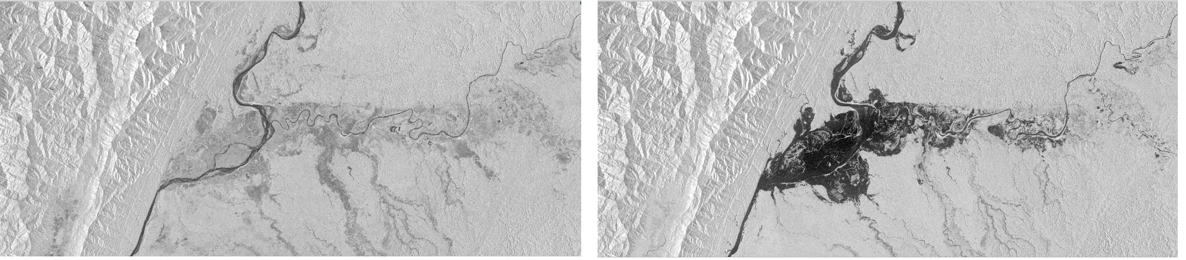
Map.addLayer(VV_pre,  {'min': [-30], 'max': [0]}, 'VV Pre_flood '+str(date_pre_flood)) # To appear as new project layers 
Map.addLayer(VV_post, {'min': [-30], 'max': [0]}, 'VV Post_flood '+str(date_post_flood))

The VV polarisation images before and after the flood will appear as new project layers that we can enable and disabled as normally done when working in QGIS, providing the follwing results:

An RGB composite with the pre-flood image in the red channel, and the post-flooding image in the blue and green channels:

# RGB of change
RGB=VV_pre.addBands(VV_post)
RGB=RGB.addBands(VV_post)
Map.addLayer(RGB, {'min': [-20,-20,-20], 'max': [0,0,0]}, 'RGB: [pre,post,post]')

Resulting in: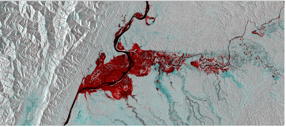

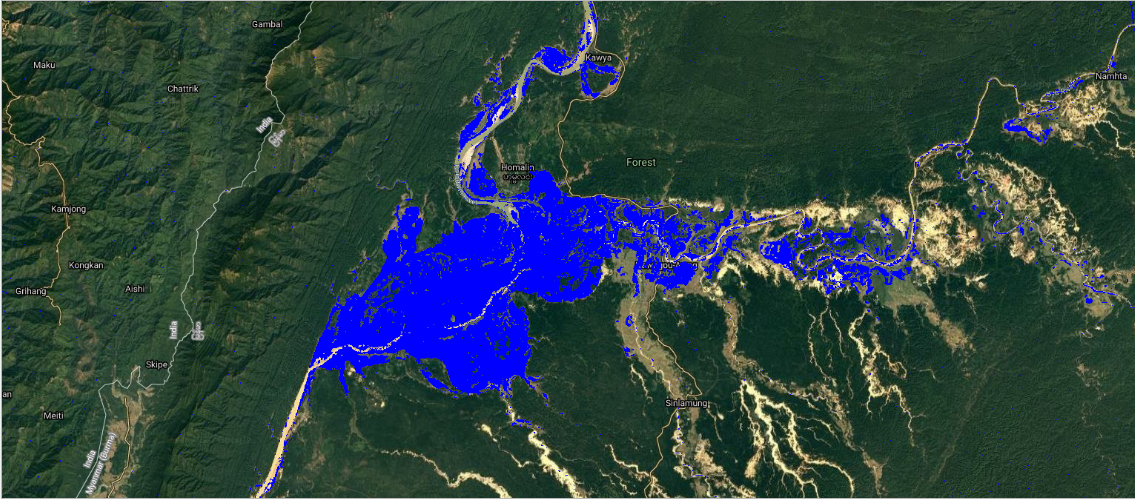
We can obtain a mask of the flooded pixels by analysing the ones that changed significantly between the pre and post flooding images. We do this im this case as suggested here, by simply computing the difference between them and setting a threshold corresponding to the limit where we consider that a change in backscatter greater than this limit, was caused by the flooding event and not by other natural causes. In the following example, a change of more than 4 dB between images is considered to have been caused by the flooding:

Diff_upper_threshold=-4 # 4 db threshold
#Threshold smoothed radar intensities to identify "flooded" areas.
Smoothing_radius = 100
diff_smoothed = (VV_post.focal_median(Smoothing_radius, 'circle', 'meters')
.subtract(VV_pre.focal_median(Smoothing_radius, 'circle', 'meters')))
diff_thresholded = diff_smoothed.lt(Diff_upper_threshold)
Map.addLayer(diff_thresholded.updateMask(diff_thresholded), {'palette':["0000FF"]},'Flooded areas mask')

Note that the selection of this threshold can vary from a subjective decision, complex statistical anlysis of all the pixels in the images, and several other methods. In fact, this problem has been intensively studied by the remote sensing comunity for the change detection applications and we will be looking at some of them in a future post. After masking the flooded pixels, we obtain:

Translating the same methodology to other test sites is just a matter of changing the parameters to filter the image collection in the GEE platform. Replicating this example for a flooding occured this year in England is done by first updating the following parameters:

##############################
######### England ############
##############################
dates_pre_flood =['2020-02-10','2020-02-24'] # dates 
dates_post_flood=['2020-02-24','2020-03-15']
map_center=[52.669613,-2.632745] 
Direction = "DESCENDING"
orbit_No  = 154# 

Which results in: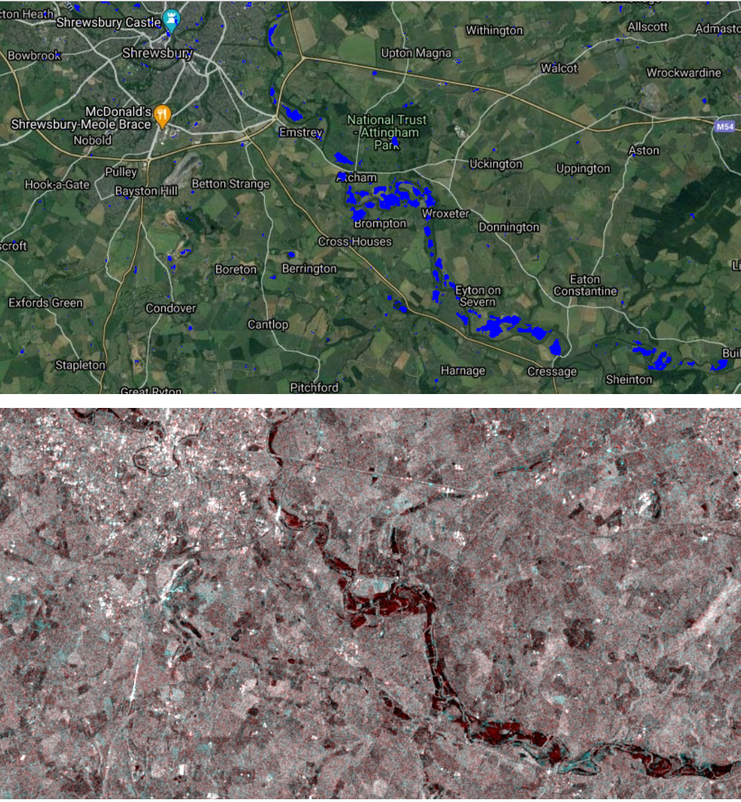

Note that because we are directly obtaining these results as project layers, creating a more comprehensive map is a straightforward process as explained for example in this tutorial.

… Under construction …